Introduction
Popular events, breaking news, and other happenings around the world drive hundreds of millions of visitors to Twitter, and they generate a huge amount of traffic, often in an unpredictable manner. Advertisers seize these opportunities and react quickly to reach their target audience in real time, resulting in demand surges in the marketplace. In the midst of such variability, Twitter’s ad server — our revenue engine — performs ad matching, scoring, and serving at an immense scale. The goal for our ads serving system is to serve queries at Twitter-scale without buckling under load spikes, find the best possible ad for every query, and utilize our resources optimally at all times.
Let’s discuss one of the techniques we use to achieve our goal:
A brief overview of the ad serving pipeline
A brief introduction to the ad serving pipeline (henceforth called serving pipeline) is in order before discussing the technique in detail. The serving pipeline can be visualized as a funnel with the following stages:
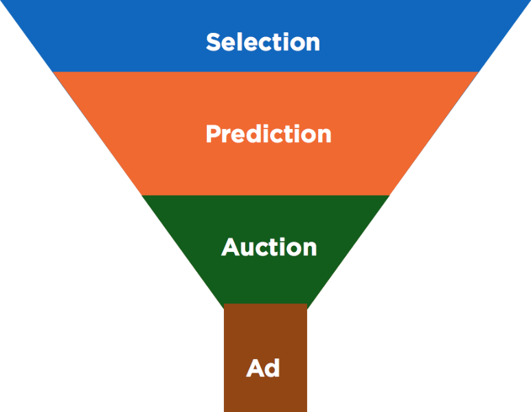
Selection
The selection phase sifts through the entire corpus of potential ad candidates for a query and comes up with a set of matches whose targeting criteria match the user in question. Selection may result in as little as a few tens to as many as several thousands of candidates being selected. All these candidates are eligible participants in subsequent stages. The number of ad candidates selected for a particular query is essentially the result of a match between user attributes and targeting criteria across the corpus of ads in the index. Hence, not all ads are relevant for all users.
Engagement rate prediction
The engagement rate for an ad is defined as the ratio of the number of engagements (e.g., click, follow, Retweet) on an ad impression to the total number of impressions served. Engagement rate is a critical predictor that determines the relevancy of an ad for a particular user (this score can be used to answer the question, “How likely is user U to engage with ad A?”). This rate changes in real time, and is evaluated by machine-learned models based on a number of user and advertiser features.
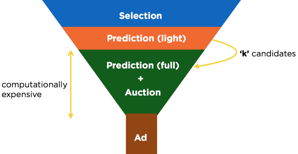
Evaluating the engagement rate is one of the most computationally expensive phases of the serving pipeline, and therefore, we run multiple rounds of this predictor to progressively thin down the number of candidates that are ultimately run through the auction. We first run a light version of the predictor over the entire set of selected auction candidates. We use this to limit the number of candidates to some top-k (order of hundreds) that we then run through the full auction. Since the best ad can be found by running all the selected candidates through the auction, it stands to reason that by decreasing the value of k, we make the auction cheaper in terms of both CPU utilization and latency, but at the same time find a slightly lower-quality ad. Therefore, k serves as a knob that can be used to tradeoff latency against ad quality.
Auction
Typically, a standard second-price auction is run for every request on the expected cost per impression (computed as bid times the engagement rate). Additional rules and logic apply if the bidding happens on our ad exchange, Mopub marketplace.
Ad server latencies and success rate
Queries hitting the ad server are not all the same in terms of how valuable they are; some queries are more monetizable than others, thereby making the cost of a failed query variable. Requests also have high variance in compute, depending upon the ad match. We observe two strong correlations:
High latency requests — the ones that influence success rate — therefore contribute disproportionately to revenue. Simply put, the more work we expend for a query, the more revenue we stand to make. Hence it follows that timing-out the higher latency requests has a disproportionately negative impact on revenue. We can conclude from the above observation that it is very important to maintain a high success rate.
Using k to scale the ad server
As you will recall, k is a knob that can be used to control CPU utilization and latency. This provides us with an interesting insight — we could simply use k as a means to scale the ad server, as long as we have a good way to pick the right value for k for every query.
One strategy to pick k is to predictively determine its value based on a set of observable features for every query (e.g., current load, available CPU, current success rate, user features, etc.). While this approach is promising, it is expensive and hard to model precisely. Our model(s) for predicting k would have to be complex to react quickly to external parameters (e.g., load spikes), and such prediction itself can prove to be computationally expensive.
Another strategy is to continually learn the value for k. To do this, we should pick a metric to center the system around that’s both fundamentally important to the system as well as influenced directly by this knob, k. Since we know that k directly influences latency, an adaptive learning strategy that learns k by tracking success rate is a viable approach.
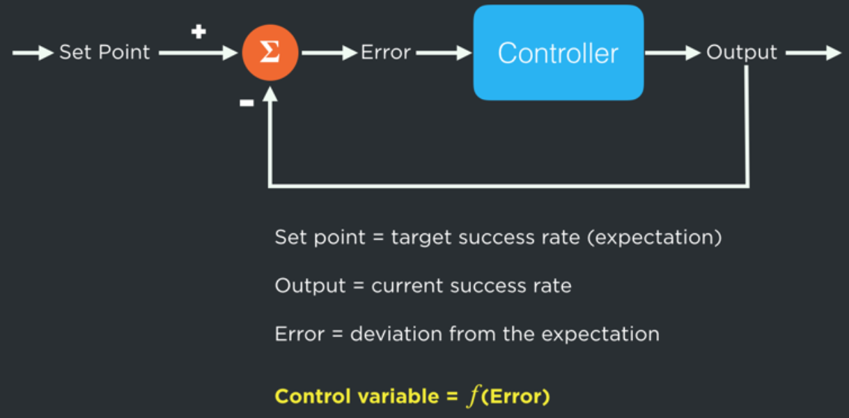
We build this adaptive learner into our ad server, which essentially functions as a control system that learns k. For quick reference, a basic controller (see figure below) keeps a system at a desired set point (expectation) by continuously calculating the deviation of the process output against the set point through a feedback loop, and minimizes this error by the use of a control variable. Mapping this to the ad server’s goal of operating at the right k value, we fix our set-point to the target success rate we desire (say, 99.9%), and build a controller that constantly tracks towards this success-rate by adjusting k.
QF: adaptive quality factor
The controller we build outputs a control variable called quality factor (q), which performs the function of keeping the success rate (SR) at the expectation. q varies by following a few simple rules. q reduces by some δ for every failure, and increases by f(δ) for every successful query. For example, if the target SR is to be kept at, 99.9%, every failure will reduce q by δ, and every successful query will increase q by δ/999. Hence, if the system stays at the target success rate of 99.9%, the variation of q within the span of 1,000 requests would be negligible. δ and f will determine the rate at which q will adapt, and can be set with proper tuning.
Any target success rate can be translated into a target latency requirement since latency and success rate are inversely related. If our target SR translates to a target latency requirement of T, we can say that in effect, q stays constant as long as we are at the target latency. It increases when the latencies are lower than T, and decreases when the latencies exceed T. When the ad server starts, it picks some default value for q which then adjusts to a level commensurate with the current load and latency profile by following the aforementioned rules.
How do we use q?
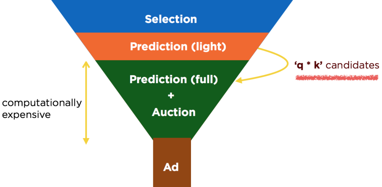
With q defined as above, we select the top q*k candidates after our light prediction stage instead of k, q converges when query latencies are around T. During times of high QPS or failover, q automatically adapts down, thereby reducing the number of candidates entering the full auction and reducing the load on a computationally expensive step (while suffering a loss in ad quality). This consequently reduces query latency, and keeps our success rate to upstream clients on target. Importantly, during regular operation, we can operate at a q value of greater than 1.0 with current provisioning (since we provision for DR, and have extra capacity available most of the time).
The figure below shows how q adapts to variation in load (both are normalized by some factor to show the interplay more clearly). During times of low qps, q trends up, thereby effectively increasing the amount of work done per query, and when qps peaks, q trends down, reducing the work done per query. This has the effect of using our CPU optimally at all times.
Another interesting aspect of this design is that each ad server instance maintains its own view of an optimal q, thereby ensuring that we have resiliency at a local, per-instance level, requiring no central coordination.

In practice, the ad server uses several tunable parameters to control the performance characteristics of various parts of the system. The k we saw before (candidates after light prediction) is only one such knob. We can now use q as a parameter to tune each of these other parameters further, thereby achieving efficiencies across the whole of the ad server.
You might recollect that at the beginning of this blog, we stated that our goal was around effectively utilizing CPU, but our technique of using the quality factor tried to achieve this goal by ultimately controlling latency. In order for this to improve CPU utilization, we would have to first ensure that the ad server is CPU bound, and not latency bound. We achieve this by making all operations asynchronous, reducing lock contention, etc.
How does q help with provisioning?
The typical approach to provisioning is to allocate resources at a level such that comfortably allows for temporary spikes in load and maintain business continuity during failovers (disaster recovery).
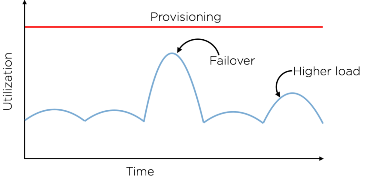
It is easy to see why this is wasteful, since we end up underutilizing resources during the normal course of operation. Ideally, we would like for our utilization to always be close to our provisioning, while still being able to absorb load spikes (as shown in the green line in the curve below):
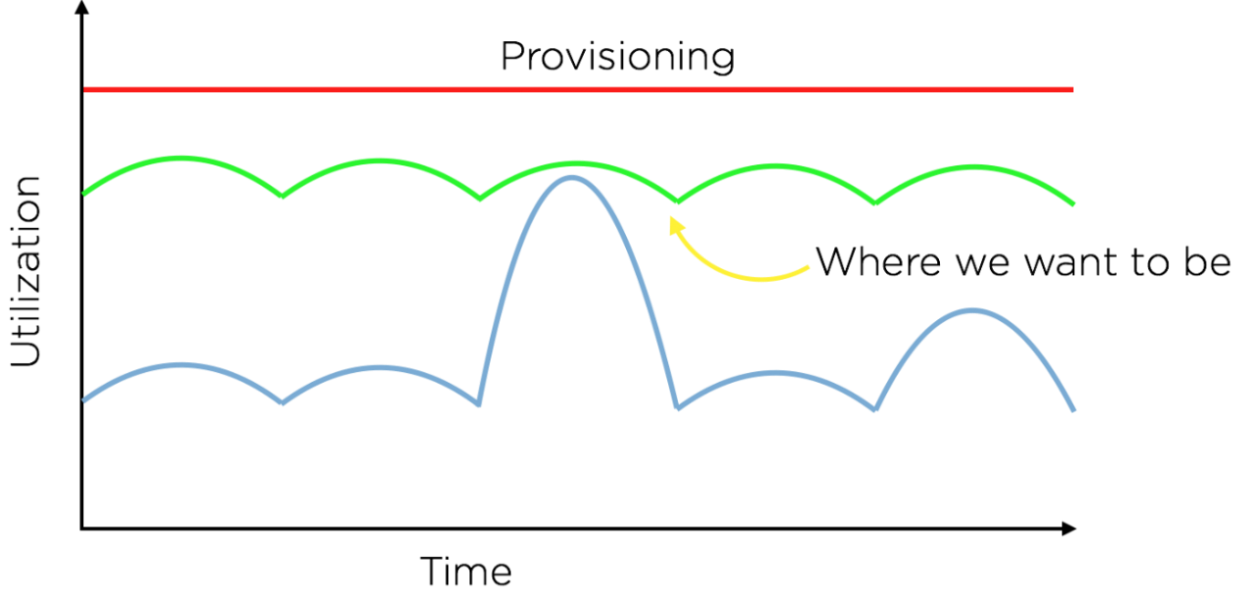
Quality factor helps us understand and maintain optimal provisioning levels. With experimentation, we are able to measure the impact of varying q on key performance indicators such as RPMq*, and also on the impact on downstream services (during query execution, the ad server calls out to several downstream components such as user-data services and other key-value stores. The impact on these downstream components should, therefore, be taken into account for any provisioning changes in the ad server). Thus, we’re able to increase or decrease our provisioning levels based on desired operating points in our system. By directly controlling utilization, q allows us to use our provisioning optimally at all levels.
This benefit, however, does not come without cost. As alluded to before, we trade off ad quality for this ability to always optimally utilize our resources. Since q basically tracks ad quality, we see a temporary dip in ad quality during periods of high load. We see in practice that this is a very fair tradeoff to make.
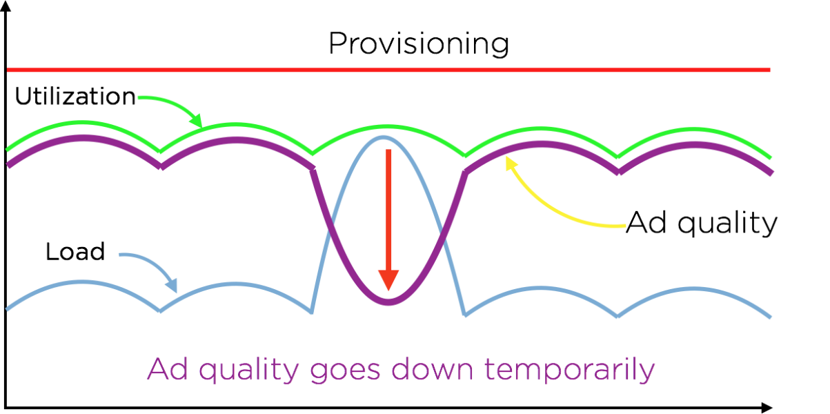
Since q semantically represents the revenue made per unit core time, it also serves as a ready metric for us to get a sense of current performance from a revenue (or more precisely, an RPMq) standpoint. This graph shows the strong correlation:

Wrapping up
The technique we’ve outlined uses concepts from control theory to craft a control variable called quality factor, which is then used by the ad server in achieving the stated goals around resiliency (availability), scalability, resource-utilization, and revenue-optimality. Quality factor has benefited our ad serving system enormously, and is a critical metric that is now used to tune several parameters across the ad server besides the auction depth. It also allows us to evaluate the cost of incremental capacity increases against the revenue gains they drive.
The ads serving team at Twitter takes on challenges posed by such enormous scale on a continual basis. If building such world-class systems excites you, we invite you to join the flock!
Acknowledgements
Ads Serving Team: Sridhar Iyer, Rohith Menon, Ken Kawamoto, Gopal Rajpurohit, Venu Kasturi, Pankaj Gupta, Roman Chen, Jun Erh, James Gao, Sandy Strong, Brian Weber. Parag Agrawal was instrumental in conceiving and designing the adaptive quality factor.
*RPMq = Revenue per thousand queries.
Did someone say … cookies?
X and its partners use cookies to provide you with a better, safer and
faster service and to support our business. Some cookies are necessary to use
our services, improve our services, and make sure they work properly.
Show more about your choices.