In previous posts, we discussed how A/B testing helps us innovate, how DDG, our A/B testing framework, is implemented, and a technique for detecting bucketing imbalance. In this post, we explore and dismiss the idea of using a second control to reduce false positives.
The trouble with probabilities
A/B testing is a methodology fundamentally built on a framework of statistics and probability; as such, the conclusions we reach from experiments may not always be correct. A false positive, or a type I error, is rejecting the null hypothesis when it is actually correct — or, roughly, claiming that a behavior change is seen when in reality there is no change between the sampled populations. A false negative, or type II error, is accepting the null hypothesis when it is actually not correct — in other words, claiming that we don’t see a change between the buckets when a difference exists between sampled populations.
A well designed statistical experiment aims to minimize both types of errors. It is impossible to completely avoid them. Naturally, this uncertainty can be very concerning when you are making ship/no-ship decisions, and you are not sure if the changes you observe are “real.”
This post will examine the idea of using two control buckets in order to guard against these errors. We will demonstrate this causes significant problems, and that creating a single large control is a superior and unbiased way to achieve the same goal using the same amount of data.
Testing with a second control
An A/A test is one in which no changes are applied to the “treatment” bucket, effectively resulting in having two controls. A/A tests are a very useful tool for validating the testing framework. We regularly use A/A tests to verify the overall correctness of our tooling: to see if the statistical methods are implemented correctly, check that there are no obvious issues with outlier detection, and spammer removal. A/A tests can also be used to determine the amount of traffic necessary to detect predicted metric changes.
Some experimenters at Twitter proposed running A/A/B instead of A/B tests, to reduce the false positive rate due to “biased” buckets. An A/A/B test is one in which in addition to the provided control (A1), an experimenter would add another control group (A2) to their experiment.
There are two approaches to using the two control buckets. The first approach is to use A2 for validation — if treatment shows significant differences against both control A and control A2, it is “real”; otherwise, it’s discarded as a false positive. Another approach is to use A2 as a replacement control when A1 bucket is believed to be a poor representation of the underlying population.
Our analysis shows that both of these approaches are inferior to pooling the traffic from the two controls, and treating it as a single large control — in other words, if you have the traffic to spare, just make your control bucket twice as big.
Statistics behind the second control
Let us consider the possible outcomes of an A/A/B test in which the reality is that the null hypothesis is true and treatment (B) has no effect.
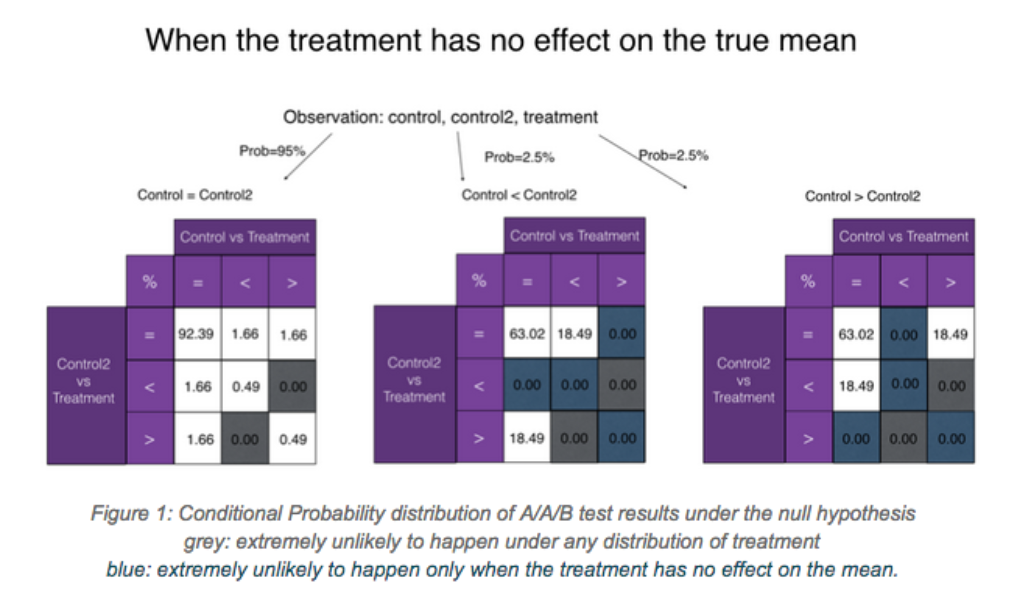
Below, we present all possible combinations of significance outcomes between the three buckets. At significance level of 0.05, there is 95% chance of seeing non-significance between A1 and A2 (the left diagram). Among the remaining 5%, half of the time A1 will be significantly smaller than A2, and half of the time the reverse will hold (the middle and right diagrams).
The number in each cell is the percent of the time a particular combination of A1 vs Treatment and A2 vs Treatment occurs, given the A1-A2-B relationship. These values are analytically derived; you can find the derivation in the appendix.

We will now examine both approaches to using two controls, and show why they are suboptimal compared to combining both control buckets into a single large control.
Analysis of Approach 1: rejecting upon any disagreement
Recall that the first approach states that we accept the null hypothesis unless it is rejected when comparing against each of the controls. We also discard all results in which controls disagree.
Controls will disagree in 5% of the cases by construction, and those are thrown out immediately.
Per the leftmost table in Figure 1, the chance of observing both controls being significantly different from treatment under the null hypothesis (two false positives in a row) is merely 0.49% + 0.49% = 0.98% of 95%, or 0.93% of the total. Thus the rate of false rejections of the null hypothesis is significantly reduced, from 5% to under 1%.
This comes at a price. Using two controls, either of which can cause the experimenter to accept the null hypothesis, is a much stronger requirement that will cause false negatives in cases where B does indeed diverge from control. We drop power by introducing this constraint, which results in a sharp increase to the false negative rate.
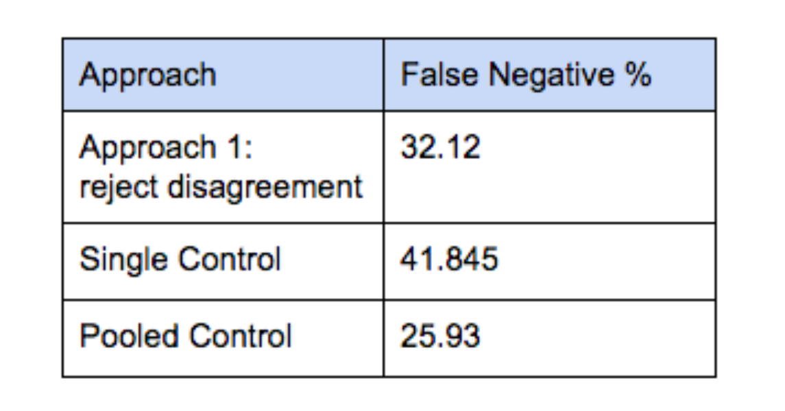
The specific false negative rates depend on how much a treatment moves the metric. By way of illustration, we consider a normal distribution with mean of 0 and standard deviation of 1 in both controls, and mean of 0.04 and standard deviation of 1 in treatment. The table below presents the false negative % that can be analytically derived using the same methodology as presented above. We compare it to simply using a single control and to using a pooled control. P-value is set to 0.0093 in both cases in order to match Approach 1’s false positive rate.

In all cases, one pays a very high false negative cost for such a low false positive rate. While Approach 1 outperforms using a single control, it produces many more false negatives than does combining the traffic from both controls into a single large pooled control.
Analysis of Approach 2: pick the “best” control
The second approach for using two controls is to try to identify which of them is the best representative of the underlying population. Since we would be identifying the “best” control after seeing experiment results, this approach suffers from severe temptation to cherry-pick and make biased choices. This is a significant danger, and the biggest reason to completely avoid using two controls.

Let us be charitable, however, and imagine that instead of “going with our gut” to pick between A1 and A2, we perform analysis to determine which of the two controls is a better representative of the underlying data. Let’s further assume (unrealistically) that our analyst has access to the true distributions and can always correctly identify the best control.
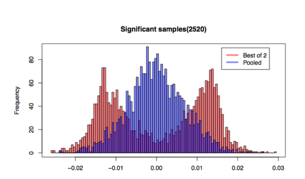
We simulate 50,000 pairs of (A1, A2) buckets each with 10,000 samples from the standard normal distribution. In our simulation, 2492 (4.98%) turn out to have statistically significantly different means.
Since we know the distribution from which we drew the simulated data points, it’s easy for us to to simulate a perfect “best control” oracle. For each pair of controls, we simply pick the one whose mean is closer to 0. We compare it to the mean of the pooled control, which is of course the average of the two control means — we will call it “average.”
The cases where two controls do not exhibit statistically significant differences are not interesting, since they do not cause the experimenter to choose a “best” control. Let us consider only the cases when we observe divergence between A1 and A2. From the plot below we see that “best of 2” correctly centered at zero. However, while the pooled plot appears to fit the expected unimodal shape, the “best of 2” strategy results in a bimodal back of a two-humped camel. Variance of means from the pooled approach is 4.81e-5, while variance of “best of 2” is a much higher to 1.45e-4.

The shape exhibited by “Best of 2” is not surprising if we consider what must happen in order for two controls to be seen having a statistically significant difference. Statistical significance is measured based on the difference between the two controls’ means. The further apart they are, the more different we observe them to be. Given a normal distribution of sample means (cf. Central Limit Theorem), for any difference d, the probability of seeing difference d due to two samples coming from either side of the true mean is higher than the probability of both means coming from the same side of the true mean. In other words, if you see a large difference between two controls, chances are it’s because one is (much) larger than the true mean, and the other is (much) smaller than the true mean. Averaging them will tend to give you something closer to the true mean than picking either of the extremes.
We can clearly see from this simulation that when the two control buckets diverge, pooling them provides a better estimation of the mean of the distribution with lower variance, and therefore has much higher power, than even a perfect oracle that correctly identifies the “best” control 100% of the time. Pooled control will perform even better in the real world, since correctly identifying the “best” of two controls 100% of the time is impossible.
Conclusion
Doubling the size of a single control bucket is preferred over implementing two separate t-tests using two control buckets. Using two controls exposes the experimenter to a high risk of confirmation bias. If the experimenter resists the bias and only uses the second control as a validation tool, the experiment suffers from higher rate of false negatives than if the controls were pooled. Pooling will also tend to result in a better estimate of the true mean than using just one of controls, and does not require defining a methodology for choosing the “best” control. Experimenters should be discouraged from setting up a “second control” in a misguided attempt to protect themselves against errors.
Acknowledgements
Dmitriy Ryaboy co-authored this blog post. We’d like to thank Chris Said, Robert Chang, Yi Liu, Milan Shen, Zhen Zhu, and Mila Goetz, as well as data scientists across Twitter, for their feedback.
Did someone say … cookies?
X and its partners use cookies to provide you with a better, safer and
faster service and to support our business. Some cookies are necessary to use
our services, improve our services, and make sure they work properly.
Show more about your choices.